A Practical Guide to Mapping and Interrogating Transcription Factor Binding Sites
From in silico prediction to confirmed binding: a bench-level walkthrough by someone who has stared at a luciferase readout at 11 pm and questioned their life choices.
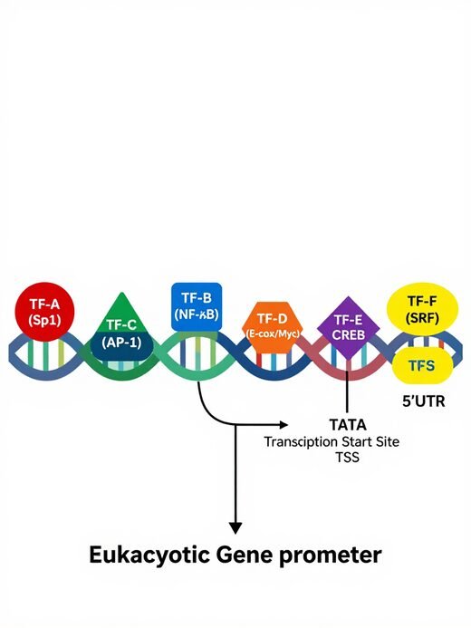
A transcription factor (TF) binding site (TFBS) is a short DNA sequence in a gene’s promoter where a TF docks to participate in switching transcription on or off. This guide walks through prediction, public ChIP-seq filtering, functional assays, and direct binding confirmation — with BondLab tools linked at each step.
Quick Orientation: What Is a TFBS and Why Should You Care?
A transcription factor binding site, or TFBS, because nobody has time to say the whole thing, is a short stretch of DNA (usually 6–20 base pairs in length) in or near a gene's promoter that a specific transcription factor recognises and physically binds to. When that TF docks on, it either recruits the transcription machinery to crank up expression, or it calls in repressors to shut things down. It might sound trivial but it can have enormous consequences for the cell.
Why does this matter to you? Because if you're asking questions like "why does my gene go up when I treat cells with Drug X?" or "what's driving expression in tumour cells but not in normal tissue?" , the answer usually traces back to a TF and its binding site in the promoter. The TFBS is where the regulatory decision gets made.
Here's the rough workflow we go through in the BondLab:
- Step 1: Predict: Use computational tools to scan your gene's promoter for known TF motifs.
- Step 2: Filter: Cross-reference with publicly available ChIP-seq data and evolutionary conservation to separate signal from noise.
- Step 3: Perturb: Knock down or inhibit the candidate TF and see if your gene changes expression.
- Step 4: Report: Clone the promoter into a luciferase reporter and dissect it with truncations and site-directed mutagenesis.
- Step 5: Confirm: Show the TF actually sits on that DNA in your cells using EMSA or ChIP.
None of these steps alone is a proof. All of them together contribute evidence that the TF is an important regulator of your gene of interest.
In Silico Identification: Scanning Your Promoter for Motifs
Before you touch a pipette, do your computational homework. You want a shortlist of candidate TFs that might regulate your gene, not a list of five hundred, which is what you'll get if you're not careful.
Getting Your Promoter Sequence: The Bond Lab Tools
First things first, you need the promoter sequence. The BondLab site has a genuinely handy tool for exactly this: Promoter Grabber lets you look up a gene by name or accession, specify how far upstream you want (say, 2 kb upstream of the TSS), pull the sequence, and export it in FASTA format ready for downstream analysis. It is refreshingly straightforward: type in your gene symbol, select your species, pick your window size, and grab the sequence. No login, no faffing about. Seriously, bookmark it.
Scanning for Motifs with FIMO
Once you’ve got your FASTA sequence, head over to the BondLab transcription factor binding site scanner or FIMO at the MEME Suite. FIMO (Find Individual Motif Occurrences) scans a DNA sequence against a library of position weight matrices (PWMs) and tells you where each TF motif appears, along with a p-value for how well the match fits the ideal motif.
Here's the basic workflow in FIMO:
- Paste or upload your promoter FASTA sequence in the input box.
- Select your motif database, we'll talk about JASPAR in a moment.
- Set a p-value threshold (more on this below).
- Hit submit and wait a few minutes.
- Download the results table and brace yourself for a wall of hits.
Where to Get TF Motifs: JASPAR
JASPAR is the place to go for an open-access database of TF binding profiles. It's curated, peer-reviewed, and covers vertebrate and non-vertebrate TFs. When you're loading a motif database into FIMO, pull it straight from JASPAR, use the JASPAR CORE vertebrates collection for most mammalian work. You can also browse JASPAR directly to look up the binding profile for a specific TF you care about, download its PWM, and use that for a targeted scan rather than scanning the whole database. Targeted scanning is almost always a better idea when you have a specific hypothesis.
Filtering the Avalanche: Practical Advice
Okay, so you've got your FIMO results table. What do you do with it now? Here's how to actually narrow it down to something useful:
P-value threshold: FIMO reports a p-value per hit. A common cutoff is 1×10⁻⁴, but honestly, tighten that to 1×10⁻⁵ or even 1×10⁻⁶ for initial filtering. The p-value here reflects match quality to the PWM, not biological relevance but higher stringency at least means the motif sequence is a closer match to the ideal.
Relative score: FIMO also gives you a score relative to the maximum possible for that motif. Aim for hits scoring above 85% of the maximum, anything lower is a very weak match.
Multiple testing correction: FIMO applies a q-value correction (Benjamini–Hochberg) automatically. Filter on q-value below 0.05. It's the more honest metric.
Biological relevance check: Cross your FIMO hits against TFs that are actually expressed in your cell type. No point investigating a TF that isn't even present. Check your own RNA-seq data or look up cell type expression in the Human Protein Atlas.
Conservation as a filter: We'll cover this properly in Section 4, but the short version is: a predicted binding site that's also conserved across species is far more interesting than one that's unique to your species.
The single most important filter isn't the p-value, it's biological context. If you already have clues about which pathway is involved (from your perturbation data, from the literature), prioritise motifs for TFs in that pathway. Hypothesis-driven filtering beats brute-force scanning every time. Let the biology guide which computational hits you follow up.
Mining Public ChIP-seq Data: ENCODE and BEEP
Here's a gift that earlier generations of molecular biologists didn't have: massive amounts of publicly available ChIP-seq data telling you exactly where thousands of TFs are bound across dozens of cell lines. Before you do a single experiment, you can check whether your TF of interest is already known to bind near your gene. This is genuinely one of the most powerful filtering steps available, and a shocking number of people skip it.
The ENCODE Project
The ENCODE (Encyclopedia of DNA Elements) project has generated ChIP-seq datasets for hundreds of TFs across many human and mouse cell lines. The data is freely accessible, well-curated, and searchable. You can find ChIP-seq peaks for your TF of interest in a relevant cell type, download the peak file, and check whether any peaks land near your gene's promoter.
BEEP: A Friendlier Interface for ChIP Data
Navigating raw ENCODE data can be a bit overwhelming. That’s where B.E.E.P. (BondLab ENCODE Enabled Promoters) comes in. See the B.E.E.P. user guide for a full walkthrough. B.E.E.P. provides a streamlined interface to query ENCODE ChIP-seq data and asks essentially this question: “Is my TF of interest bound near my gene of interest in a relevant cell type?” You put in a gene name, choose a TF, pick a cell line, and it tells you whether there’s a ChIP-seq peak in that region. It’s a huge time-saver compared to manually wrangling ENCODE downloads.
Cross-Species Conservation: A Hint, Not Proof
Evolution is your friend here. If a short sequence in your promoter has been maintained across millions of years of evolution, across mouse, rat, dog, cow, maybe even chicken, there's a pretty good argument that natural selection kept it around because it does something important. Most random mutations in promoter regions are tolerated. Conserved sequence = likely functional.
To check conservation, fire up the UCSC Genome Browser or our BondLab genome browser. Both are free and comprehensive. Alternatively, try the BondLab cross-species TF scanner. Navigate to your gene, look at the promoter region, and turn on the PhyloP or PhastCons tracks (found under the Comparative Genomics section). PhyloP scores individual nucleotide conservation; PhastCons scores conserved elements. A cluster of high PhyloP scores sitting right on top of your FIMO-predicted TFBS is very encouraging.
For a more visual, alignment-based view, try the VISTA Browser. It's excellent for seeing blocks of conserved sequence between your species and others, rendered as a sliding-window conservation plot. It makes it easy to see whether your predicted site sits inside a conserved peak or out in a divergent wasteland.
Conservation is a filter, not proof. Some entirely species-specific binding sites are biologically important, particularly in cases of lineage-specific gene regulation or in regulatory evolution. Some conserved sequences are structural/architectural elements that don't contain TF binding sites at all. Use conservation to prioritise, not to conclude. A conserved TFBS prediction from FIMO with a nearby ENCODE ChIP-seq peak is a strong candidate but it still needs functional and binding validation before you can claim it means anything.
Functional Assays: Does the TF Actually Drive Expression?
Alright, you've got one or a few candidate TFs with predicted binding sites in your promoter, some ChIP-seq support, maybe some conservation. Now it's time to ask: does this TF actually control transcription of your gene in a live cell? There are three main routes to answering that question.
Route 1: Pharmacological Inhibition of the TF
The quickest and dirtiest approach is to inhibit the TF with a small molecule and measure whether your gene goes up or down. Classic examples include JQ1 (a BET bromodomain inhibitor that particularly targets BRD4 and displaces it from chromatin), various NF-κB pathway inhibitors like BAY 11-7082 or IKK inhibitors, or SP600125 for AP-1/JNK signalling.
Pharmacological inhibitors are never perfectly specific. JQ1 inhibits all BET proteins (BRD2, BRD3, BRD4, BRDT), not just BRD4. NF-κB inhibitors often hit other signalling components. If your gene changes after inhibitor treatment, that's interesting and worth pursuing but you cannot conclude BRD4 specifically, let alone a specific binding site. Think of pharmacological data as directional evidence, not mechanism.
Route 2: Genetic Knockdown or Knockout of the TF
This is more convincing. Use siRNA, shRNA, or CRISPRi to specifically reduce expression of your candidate TF, then measure your target gene by qPCR or RNA-seq. A meaningful drop (or rise, for repressors) in your target gene after TF knockdown strongly suggests a regulatory relationship.
A few things to do well here: use at least two independent siRNA/shRNA sequences targeting different regions of the TF mRNA. This helps to guard against off-target effects. Confirm knockdown efficiency (both at mRNA and protein level: western blot your TF). Include a non-targeting scramble control. Measure your target gene by RT-qPCR with validated reference genes, or if you're doing RNA-seq, do it properly with biological replicates and DESeq2 or edgeR.
CRISPRi (dCas9-KRAB) targeting the TF gene itself is increasingly the gold standard here. You get tight, inducible, reversible knockdown without the off-target issues of RNAi. If your lab has a dCas9-KRAB cell line, use it. It'll make reviewers happier.
Route 3: Reporter Assays - the Workhorse of Promoter Biology
This is where you get to dissect the promoter itself. You clone your promoter upstream of a reporter gene, usually Firefly luciferase or nanoluciferase, transfect it into your cells of interest, and measure reporter activity. This is the most direct test of whether a given DNA sequence has promoter activity, and whether specific elements within it matter.
The logic is simple: if the sequence drives reporter expression, it's a functional promoter. If mutating a predicted TFBS drops reporter activity, that site is functionally important. Honestly, when it works, it's one of the most satisfying experiments in molecular biology.
Truncation Analysis (5' Deletion Series)
Start by cloning a big chunk of promoter, say 2 kb, upstream of the reporter gene (in the BondLab we regularly use nanoluciferase reporters due to their fantastic sensitivity) Then make a series of 5' deletions: 1.5 kb, 1 kb, 500 bp, 250 bp, 100 bp upstream of the TSS. Transfect each construct into your cells, measure the reporter activity, and plot activity against length. When you see a big drop between two adjacent constructs, say activity halves between the 500 bp and 250 bp construct, you've just localised a critical regulatory region with a net positive activity (because when you delete it activity goes down) to that 250 bp window. If the activity goes up the region you deleted has a net negative activity. Remember that a region of 200 or more bp probably contains many TFBS, so the activity change you observe is the result of the sum of all these factors. You may need to make a new series of more detailed truncations to narrow down the search for the important motif. Now you know where to look for your TFBS.
Design your deletion boundaries to not cut through predicted TFBS motifs. If you want to resolve whether site A (at −320 bp) or site B (at −280 bp) is responsible, your deletion boundaries need to fall between them. Map your FIMO hits first, then design your truncations to bracket them cleanly.
Site-Directed Mutagenesis of the Predicted TFBS
Once truncation analysis has pointed you to a region, mutate the specific bases that FIMO predicts are critical for TF binding. How do you design a good mutant? Look at the position weight matrix for your TF, the columns with the highest information content (the most conserved positions in the motif) are the ones to mutate. Change those bases to something as divergent as possible from the consensus. If the consensus is GCGGGGCG, don't just change one G to A, swap the highest-information-content positions to their worst-match bases. A double or triple point mutant at the core of the motif is more convincing than a single mutation.
Critically: design your mutant so it doesn't create a new predicted binding site for a different TF. Run your mutated sequence back through FIMO and check that you haven't accidentally introduced a high-scoring motif for something else. It happens more often than you'd expect and it makes for very confusing results.
Normalisation, Controls, and Statistics
A few important practices for reporter assays:
Co-transfect a Renilla luciferase construct (like pRL-TK) to normalise for transfection efficiency. Report firefly/Renilla ratios, never raw firefly values.
Include a promoterless vector control (your backbone with no insert) to establish your baseline noise.
Include a positive control — a strong constitutive promoter (CMV or SV40) to confirm your transfection worked.
Biological replicates: at least three independent transfection experiments (different days, fresh plasmid dilutions, cells at different passage). Technical triplicates within an experiment are not the same thing — don't confuse them.
Transfect in the right cell type. This sounds obvious. People mess it up constantly. A promoter that's active in hepatocytes might be completely silent in HEK293 cells. Your reporter assay needs to be done in cells where your target gene is actually expressed and regulated.
Read the BondLab reporter gene assays guide.
Confirming Direct Binding: EMSA and ChIP
Reporter assays and knockdown experiments tell you that a TF influences transcription. But they don't technically prove the TF physically sits on the DNA sequence you think it does. For that, you need binding assays. There are two main ones: EMSA and ChIP.
EMSA: Electrophoretic Mobility Shift Assay
See TheBondLab top 10 tips for successful EMSA. The EMSA is a old technique but still a useful one. You design a short double-stranded oligonucleotide (typically 25–40 bp) that spans your predicted TFBS. You label it, traditionally with 32P, but chemical (e.g. biotin) labelling is increasingly popular and doesn't require radioisotope handling. You mix it with nuclear extract (or purified/recombinant protein). If the TF binds, it forms a protein-DNA complex that migrates more slowly through a native polyacrylamide gel than free DNA, it "shifts." Hence the name.
To make the EMSA convincing, you need several controls:
Cold competition: Add an excess of unlabelled oligo with the same sequence. It should compete away the shift, the band disappears or diminishes. This confirms specificity; the TF is binding the labelled oligo, not just sticking to it non-specifically.
Mutant oligo competition: Use an excess of unlabelled oligo bearing your site-directed mutations. It should NOT compete efficiently, because the TF can no longer bind it well. This is the most elegant control.
Supershift with antibody: Add a TF-specific antibody to the binding reaction. If the correct TF is in the shifted complex, the antibody will bind the TF-DNA complex and cause it to shift even further up the gel, a "supershift." This is the most direct evidence of which protein is in the complex. Use an antibody that recognises native protein (not just denatured), and use a control IgG to show the supershift is specific.
EMSAs are beautiful in theory and fiddly in practice. Nuclear extract quality is very important. If it's been freeze-thawed too many times or was prepared sloppily, you won't see clean shifts. The first time you do an EMSA, it probably won't work. The second time it might work but look terrible. By the fifth attempt, you'll understand what conditions your specific protein and cell type need. Keep a detailed protocol notebook. The small details (salt concentration in the binding buffer, incubation time, gel temperature) matter enormously.
ChIP: Chromatin Immunoprecipitation
ChIP is probably the best assay for showing TF occupancy at a specific locus in living cells. In a ChIP experiment, you crosslink protein-DNA complexes in intact cells (typically with formaldehyde), shear the chromatin to fragments of a few hundred base pairs, immunoprecipitate with an antibody against your TF, reverse the crosslinks, and then quantify whether your gene's promoter region is enriched in the immunoprecipitate.
For a targeted ChIP experiment, you then do ChIP-qPCR: design primers flanking your predicted TFBS (amplicon around 100–150 bp), run qPCR on the ChIP DNA, and compare enrichment (your TF IP) to a control IP (IgG or an unrelated antibody) and an input control. Express results as percent input or enrichment over IgG. A meaningful, reproducible enrichment e.g. five-fold or more over IgG at your specific region is compelling evidence of direct binding in vivo.
Antibody Quality: The Inconvenient Truth
ChIP only works if your antibody is good. This is honestly the most underappreciated variable in all of ChIP biology. A poor antibody gives you no enrichment (false negatives) or enriches everywhere non-specifically (false positives). Before committing to a ChIP experiment, validate your antibody: confirm it pulls down the right protein by western blot from your cell lysate. Check if it has been validated for ChIP by the manufacturer. Look up whether other labs have published ChIP with this exact antibody, that's the best endorsement.
System-Wide Analysis: Which TF Drove That Gene List?
Sometimes the question is flipped. Instead of starting with a gene and asking "which TF regulates it?", you're starting with an RNA-seq dataset, a list of differentially expressed genes, and asking "what TF(s) could explain this pattern?" This is a common situation after a perturbation experiment, and it's where systems-level tools shine.
ChEA3: TF Enrichment Analysis
ChEA3 (ChIP-X Enrichment Analysis 3) is one of the best tools for this. You paste in your list of differentially expressed genes, hit submit, and ChEA3 ranks candidate transcription factors that are most likely to have driven the expression changes. It does this by comparing your gene list against multiple integrated datasets, ENCODE ChIP-seq, ARCHS4 coexpression, GTEx, literature-curated TF-target databases, and more. The output is a ranked list of TFs, with ensemble scores integrating evidence across databases.
ChEA3 is genuinely one of the more useful recent additions to the TF analysis toolkit. Submit your upregulated genes separately from your downregulated genes — TF activators and repressors live in different parts of the output. Pay attention to the consensus rank rather than any single database's rank; TFs appearing near the top across multiple underlying databases are your most reliable candidates.
Other Complementary Tools
A couple of other tools worth knowing:
Enrichr: a broad enrichment analysis platform that includes TF libraries (ENCODE TF ChIP-seq, JASPAR TF binding) among many other gene set databases. Great as a first pass. Plug your gene list in and see which TF targets are enriched.
oPOSSUM: analyses which TF binding sites are statistically over-represented in the promoters of your gene list compared to a background set. It's older but complements ChEA3 nicely by working directly from sequence rather than from experimental datasets.
The smart approach is to run all of these, look for TFs that appear as hits across multiple tools, and then loop those candidates back into the experimental pipeline: reporter assays, knockdown, EMSA/ChIP. Computational hits are hypotheses. Validation experiments are answers.
De Novo Motif Discovery
One more powerful approach when you have a gene set: instead of scanning for known motifs, discover what motif is actually enriched in the promoters of your co-regulated genes. HOMER (Hypergeometric Optimization of Motif EnRichment) and the broader MEME Suite (including MEME for motif discovery) can do this. You extract the promoter sequences of all your differentially expressed genes, run HOMER or MEME, and let the algorithm find what sequence motifs are significantly enriched compared to background promoters. If the discovered motif matches a known TF in JASPAR, great — you have a hypothesis. If it’s novel, that’s interesting in its own right (though rarer and more difficult to follow up).
Common Mistakes
Over-relying on in silico prediction. Finding a motif in a promoter sequence is not a result. It's the start of a hypothesis. No journal worth publishing in will accept computational prediction alone as evidence of a functional TFBS.
Using a bad ChIP antibody. Validate it before committing three weeks of experiments to it. Check Antibodypedia, check the manufacturer's ChIP validation data, check the literature. If it fails by western blot, it'll fail by ChIP.
No biological replicates in reporter assays. Three wells on the same plate is three technical replicates. Three separate transfection experiments on three different days is three biological replicates. You need the latter. Reviewers know the difference and so does statistics.
Transfecting the wrong cell type. Your reporter construct will behave differently in every cell line. Pick the cell type where your biology actually happens and transfect there, even if it's harder to transfect.
Not designing proper EMSA controls. An EMSA shift with no cold competition, no mutant competition, and no supershift is unpublishable and uninterpretable. Do it right the first time.
Ignoring the fact that TFs work in complexes. Your TF of interest might need a co-factor to bind. If your single TF knockdown only partially reduces target gene expression, look for interaction partners and co-regulators. Combinatorial control is the rule, not the exception.
Skipping the public data check. Mining ENCODE / BEEP before starting bench experiments can save you weeks. It baffles me how often this step is skipped. Do it first.
A complete TFBS story, including prediction, functional validation, binding confirmation typically takes four to eight months of focused effort for one well-supported site. If someone promises you can do it faster, they're probably cutting corners. The good news is that each step genuinely builds on the last: reporter truncations guide your mutant design, mutants guide your EMSA oligo design, EMSA guides your ChIP primer placement. When it all clicks, it feels like solving a complex puzzle.
TFBS work has a reputation for being tedious and technically demanding, and honestly, that reputation isn't entirely undeserved. The EMSA that refuses to shift, the reporter construct that drives no expression in the cell line you need, the ChIP antibody that doesn't IP anything, these are real obstacles that come up all too often. But when you get to the end and you've got a predicted site that's conserved, sits under a ChIP-seq peak, reduces reporter activity when mutated, causes target gene dysregulation when its TF is knocked down, and shows a clean supershift in your EMSA, that is airtight. That is the kind of mechanistic data that reviewers can't argue with.
Use the computational tools to work smart, not just hard. The Bond Lab tools — Promoter Grabber, cross-species TF scanner, and B.E.E.P. — plus public resources such as JASPAR, UCSC, and ChEA3 are all free, and they’re good. They exist precisely to give you a head start, so use them. Filter aggressively. Pick your two or three best candidates and commit to them fully rather than half-heartedly chasing ten.
Keep your controls tight, your replicates biological and plentiful, your cell type appropriate, and your antibodies validated. Write down every protocol deviation. The experiment that works perfectly the first time is rare. The experiment you can reproduce reliably because you kept good notes? That's science.
Good luck. Go find your binding site.
Quick-Reference Checklist: Next Steps
- Pull promoter sequence (2 kb upstream) using Bond Lab Promoter Grabber at thebondlab.net
- Run FIMO scan with JASPAR CORE vertebrates database; apply q-value and relative score filters
- Check BEEP / ENCODE for TF ChIP-seq peaks near your gene in a relevant cell type
- Visualise conservation in UCSC Genome Browser (PhyloP / PhastCons tracks)
- Cross-reference candidate TFs with your cell type's expression data
- Pharmacological inhibitor pilot (if inhibitors are available) — measure target gene by RT-qPCR
- siRNA knockdown of top 2-3 candidate TFs — confirm knockdown, measure target gene expression
- Clone 2 kb promoter into luciferase vector; run truncation series in appropriate cell type
- Design and generate site-directed mutants of predicted TFBS core bases
- Run reporters with Renilla normalisation, promoterless control, biological triplicates (n ≥ 3)
- Validate ChIP antibody by western blot before committing to ChIP experiment
- ChIP-qPCR with TF-specific antibody, IgG control, positive and negative genomic loci
- EMSA with labelled oligo, cold competitor, mutant competitor, antibody supershift
- If you have an RNA-seq gene list: run ChEA3 and Enrichr for TF enrichment analysis
- Consider de novo motif discovery (HOMER or MEME) on promoters of co-regulated genes
Key Resources
- Promoter Grabber
- BondLab TF binding scanner and FIMO (MEME Suite) — motif scanning
- JASPAR — TF binding profiles database
- ENCODE Project — genome-wide regulatory data
- B.E.E.P. — ENCODE ChIP-seq overlap analysis (user guide)
- UCSC Genome Browser — conservation, tracks, annotation
- VISTA Browser — comparative genomics visualisation
- ChEA3 — TF enrichment from gene lists
- Enrichr — broad gene set enrichment analysis
- oPOSSUM — over-represented TFBS in gene sets
- HOMER — motif discovery and ChIP-seq analysis
- MEME Suite — full suite of motif analysis tools