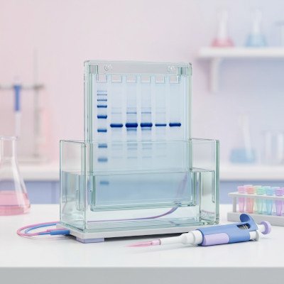
Western blot densitometry workspace with band regions marked for quantification

Western blot densitometry done properly

Related on this site: Quantify bands in the browser with our western blot densitometry tool. Upstream wet-lab advice: western blotting tips and lysis and blocking buffer recipes.

Turning a western blot into a bar graph feels routine until a reviewer asks whether the exposure was in the linear range, whether the loading control actually loaded equally, or why three lanes on one membrane count as n = 3. Densitometry is not “draw boxes and trust the software.” It is a short chain of assumptions about chemistry, imaging, background, and biology. Break one link and the numbers still look precise but they are not!

This guide is how we approach western blot quantification in The Bond Lab. From decisions on precast or home made gels, wet or semi-dry transfer, choice of membrane, normalization method and use of Bio-Rad stain-free total-protein normalization, choice of primary antibody, detection system, densitometry, signal saturation, global versus local background subtraction all matter to the final numbers you get and a workflow you can defend in review western blotting tips page.

What densitometry actually measures

A western blot reports relative antigen signal under a fixed set of conditions. How much protein you loaded, how the gel and transfer behaved, which antibody you used, how long you incubated, which substrate and imager you chose, and how hard you pushed the exposure all affect the final result. The dark band is a composite of all of that. Densitometry summarises the grey values inside a region of interest (ROI). It does not report absolute molecules of the protein being studies unless you calibrated with known standards on the same blot under the same conditions.

In our tool (and in most packages) you will see something like raw integrated optical density (IOD) and an adjusted value after background subtraction (Adj IOD). Adj IOD combines how dark the pixels are with how large the box is. That is usually what you want for a band that may smear slightly between lanes. Mean intensity ignores area, so two bands with the same average darkness but different widths are not the same amount of signal. Do not compare fat and skinny bands with mean alone.

Relative quantification answers questions like “On this membrane, is the treatment lane stronger than vehicle after normalisation?” Absolute statements such as “protein X doubled in the artery” need biological replication, a defensible loading strategy, and often orthogonal methods. Treat densitometry as evidence of a relative change on a well-run blot, not as a free-standing concentration assay.

Before you open the image

Most quantification problems start at the bench, not in the analysis software. If the blot is unevenly transferred, overloaded, or probed with an antibody that lights up half the lane, no amount of clever background subtraction will rescue it. Get the wet work right first. Our ten western tips and buffer recipes cover the usual failure modes.

Design for quantification from the start:

Load comparable amounts of total protein across lanes (or a planned dilution series if you are testing linearity).
Keep technical handling matched. Same lysis buffer, same gel percentage, same transfer sandwich, same antibody lot where possible.
Include a loading control or total protein stain that you will also quantify (see below).
Leave empty membrane for a global background box if you use that mode, and avoid writing on or touching regions you might need as background.
Plan biological replicates as separate lysates from separate experiments or animals — not three lanes from one tube.

A useful test is to run a short dilution series of a representative lysate (for example 5, 10, 20, 40 μg) on a pilot blot. If Adj IOD does not rise roughly in proportion across the range you care about, you are outside the linear response of antibody, substrate, or imager. Fix that before collecting the “real” n.

Homemade gels vs precast gels

The gel you pour (or buy) shapes resolution, transfer behaviour, and how comparable your lanes are for densitometry. Neither homemade nor precast is universally “more quantitative” — consistency within an experiment matters more than brand loyalty.

Homemade (hand-cast) SDS-PAGE gels — advantages

Cheap per gel once you own plates and a casting stand.
You choose acrylamide percentage, gradient recipes, and well format for awkward molecular weights.
Easy to cast thicker gels when you need higher protein load.

Homemade — disadvantages

Casting variability: uneven polymerisation, leaking sandwiches, and slightly different percentages between days add lane-to-lane noise that densitometry will happily turn into fake biology.
Acrylamide handling risk; you need fresh APS/TEMED and careful mixing.
Time: pouring, polymerising, and troubleshooting a crooked stack wastes an afternoon.
Harder to match commercial stain-free chemistry unless you buy stain-free acrylamide kits.

Precast gels — advantages

Batch consistency and documented shelf life; useful when several people need the same format.
Often better well geometry and fewer “smiling” artefacts if stored and run as directed.
Bio-Rad TGX Stain-Free and similar systems integrate with imagers for total-protein imaging before or after transfer (see below).
No acrylamide pouring in the open lab.

Precast — disadvantages

Cost per gel is higher, especially for stain-free or specialty gradients. A precast gel is 10 to 20 times the cost of a home made gel
Less flexible if you need an unusual percentage or comb layout.
Buffer systems are proprietary; mixing brands of gel and tank can give odd runs.
Expiry dates matter — an old cassette can look fine until transfer fails mid-project.

For quantification, pick one format for a study and stick to it. Do not mix homemade 10% gels one week with precast 4–15% gradients the next and then pool the densitometry as if nothing changed. If you must switch, re-run a bridging experiment and treat the datasets separately until you show the relative changes agree.

Bio-Rad stain-free gels and total protein

Bio-Rad’s TGX Stain-Free chemistry (and related stain-free gels) incorporates a trihalo compound in the gel that covalently modifies tryptophan residues when you activate the gel with UV (or the dedicated stain-free tray on a ChemiDoc / Gel Doc system). Proteins become fluorescent without a Coomassie or silver step. You can image the gel after the run to check load and separation, then transfer, and often image total protein again on the membrane. In Image Lab you quantify lane totals (or selected regions) as a loading control for the immunoblot densitometry that follows.

Why stain-free helps quantification

Total protein across many bands is usually a more honest denominator than a single housekeeper that may move with your treatment.
You see load and transfer problems before spending primary antibody: empty lanes, bubbles, and incomplete transfer are obvious on the stain-free image.
Same digital workflow as chemiluminescence on ChemiDoc-class imagers: activate, expose, draw lanes, export.
Avoids stripping solely to get a loading control when you would rather keep the first probe pristine.

Caveats and disadvantages

Signal depends on tryptophan content. Proteins with few Trps are under-represented; very Trp-rich proteins punch above their mass. That is fine for a whole-lane total, but do not treat stain-free intensity of a single band as a perfect mass assay.
Over-activation or very long UV exposure can affect some epitopes; follow Bio-Rad’s recommended activation times and check critical antibodies if you see odd losses.
You need a compatible imager (or UV tray) and usually Image Lab or equivalent analysis software.
Precast stain-free gels cost more than pouring classic Laemmli gels.
Stain-free total protein on the gel is not identical to protein that successfully transferred. Prefer membrane stain-free (or a membrane total-protein stain) when transfer efficiency varies across the blot.

Practical Bond Lab-style workflow: run TGX Stain-Free gel → brief stain-free activation and image → transfer → optional membrane stain-free / total protein image → block and probe → chemiluminescent (or fluorescent) capture of the antigen → in software, quantify antigen ROIs and normalise each lane to that lane’s total-protein value. Keep the stain-free exposure out of saturation just as you would for ECL. If you do not have stain-free gels, Ponceau S (documented and not over-washed) or a commercial reversible membrane stain can play a similar role — still quantify with the same densitometry rules.

Semi-dry vs wet transfer

Incomplete or uneven transfer is a classic densitometry trap: the antibody looks weaker because the protein never made it to the membrane. Choose transfer for the size of your antigen, then verify (stain-free gel after transfer, Ponceau on the membrane, or both). More bench detail is in tip 3 of our western blotting tips; here is the quantification angle.

Semi-dry transfer — advantages

Fast (often 15–45 minutes) and uses little buffer.
Convenient for mid-range proteins when the method is already validated for your target.
Less buffer mess; easy to run several sandwiches in a morning.

Semi-dry — disadvantages for quantification

Small proteins (<~20 kDa) can blow through the membrane and you under-estimate signal and lane totals look odd.
Large proteins (>~100 kDa) often transfer incompletely with residual protein left in the gel means densitometry on the blot under-reports abundance.
Local hot spots and drying artefacts if the sandwich is uneven — local background modes then fight you.

Wet (tank) transfer — advantages

Gentler and more complete for large proteins; we often run extended wet transfers (for example 2–3 h at ~400 mA) when targets are big.
Better for small proteins that need slower migration onto the membrane (sometimes with a denser membrane or brief post-transfer drying — see the tips page).
More forgiving when you care about even transfer across a wide molecular-weight range on one gel.

Wet transfer — disadvantages

Slow; more buffer; tanks heat up if you push current without cooling.
Over-transfer of very small proteins is still possible if you run too long or too hard.

Rule for densitometry: if the post-transfer gel still lights up strongly for your target region on stain-free (or Coomassie), do not quantify that blot as if load were equal. Fix transfer, then re-image.

Loading controls and total protein

Normalisation exists because pipetting, protein assay error, and transfer efficiency never match perfectly. You have three broad options: a housekeeping immunoblot, a total-protein image (stain-free, Ponceau, or commercial membrane stain), or — for phospho work — total protein for the same antigen plus a load correction.

Housekeeping proteins (GAPDH, β-actin, α-tubulin, Histone etc) are familiar and cheap once the antibody is on the shelf. They fail when the treatment changes cytoskeleton, metabolism, or cell size. In vascular smooth muscle and fibrotic models we are especially wary of actin when the phenotype itself is cytoskeletal. If the housekeeper drifts with treatment, normalisation invents or hides effects. Validate stability under your conditions, or switch strategy.

Total protein (Bio-Rad stain-free lane totals, REVERT-style stains, carefully documented Ponceau) integrates many proteins and usually tracks load better than one gene product. Quantify the denominator with the same densitometry rules as the target: same ROI discipline, same background mode, same saturation check. A pristine target band sitting on a saturated tubulin exposure is not a valid ratio.

Phospho-specific blots need an extra layer: compare phospho signal to total protein for the same antigen when you can, and still account for load. “Phospho went up” without total can just mean more protein in the lane or a change in isoform representation.

Densitometry software and workflow

All serious densitometry packages do the same core job: turn grey (or fluorescent) pixels inside an ROI into a number, optionally subtract background, and export a table. The brand matters less than using a non-saturated file and a consistent protocol.

Bio-Rad Image Lab — native path for ChemiDoc / Gel Doc and stain-free analysis; lane and band tools, saturation warnings, and reports that journals recognise.
ImageJ / Fiji — free and flexible; you must be deliberate about bit depth, background, and not accidentally applying display LUTs to the data.
Vendor software for LI-COR, Azure, Syngene, and others — fine if you stay in raw quantitative mode rather than “pretty picture” exports.
Bond Lab densitometry tool — browser-based boxes, global or local (+2 px ring) background, saturation overlay, CSV / annotated JPG export; useful for teaching and quick checks without installing ImageJ.

Recommended order of operations (any software):

Open the raw (or highest bit-depth) capture, not a Powerpoint screenshot.
Check saturation; re-expose if needed.
Straighten / crop only if required; avoid destructive contrast edits.
Choose global or local background and stick to it for the whole comparison set.
Draw comparable ROIs for antigen (and for loading control or total-protein lanes).
Export Adj IOD (or equivalent); normalise offline; archive the image with ROIs.

Manufacturer densitometry guides (Bio-Rad Image Lab tutorials, LI-COR quantitative western guides, and the papers listed below) are worth reading once so you know what your software means by “volume,” “ADJ.VOL,” or “background method.” Names differ; the ideas do not.

Exposure, bit depth, and saturation

Chemiluminescence and fluorescence imagers clip bright pixels when the detector runs out of range. Those clipped pixels all report the same maximum value, so densitometry underestimates the true difference between a strong band and a stronger one. The blot can still “look fine” on screen if display brightness is adjusted — your eyes are not a linearity check. Stain-free total-protein images can saturate too; a clipped lane total will distort every ratio that uses it.

What saturation looks like in practice: a flat white (or flat black, depending on lookup table) core inside a band, histogram pixels piled against the end of the intensity scale, or a software saturation overlay lighting up the band. On film, coal-black bricks with no grey centre are the warning sign.

Practical rules we use:

Prefer the raw capture (or the highest bit-depth export your system offers) over a heavily contrast-stretched JPEG made for a slide. Bio-Rad .SCN and similar proprietary files often preserve more than a quick PNG export.
Use saturation highlighting in Image Lab, your imager software, or our densitometry tool. If a meaningful fraction of the band (or lane total) is flagged, shorten exposure or reduce antibody/substrate and rescan.
Keep display black/white sliders for viewing only. They must not change the underlying pixel values used for quantification (our tool separates view contrast from the maths for that reason).
Avoid quantifying from a figure panel that has already been brightness/contrast edited for publication. Quantify first, then make the figure from a representative non-saturated exposure.
When target and housekeeper need very different exposures, acquire both in the linear range separately, Never normalise a gentle target exposure to a blown-out loading control.

Film has its own nonlinear response curve. If you still use film, treat densitometry with extra caution and keep exposures short enough that bands are grey, not saturated slabs.

Global vs local background and Adj IOD

Draw boxes that cover the whole band without greedily swallowing neighbouring lanes or obvious artefacts. Keep box height similar across a comparison set so you are not accidentally rewarding taller ROIs. If the image is rotated, straighten it before drawing boxes as rotating later will invalidate the ROIs (our tool clears boxes on rotate for that reason).

Background subtraction removes membrane fog and camera offset so empty membrane does not look like signal. Choosing global versus local is one of the most important densitometry decisions you make.

Global background

You mark one (or a few) empty membrane regions; the average grey from that region is subtracted from every band as if that background filled each ROI.
Best when the blot background is even, clean washes, uniform ECL, no gradient from top to bottom.
Advantages: simple, reproducible, easy to explain in methods (“global background from an empty lane region”).
Disadvantages: if background is lighter on the left and dirtier on the right, a single global value under- or over-corrects some lanes and can create fake fold-changes.

Local background

Software estimates background next to each band — for example a thin ring just outside the ROI (our tool uses a +2 px ring) or user-drawn patches beside each lane.
Best when there is a gentle background gradient, uneven ECL pooling, or you cannot find one clean global patch that represents the whole membrane.
Advantages: adapts per band; often rescues blots that would be unfair under a single global value.
Disadvantages: if lanes are packed tight, the local ring can clip the neighbouring band or a smear and invent “background” that is really signal. Speckles next to a band also poison the estimate.

Pick one mode for every lane in a comparison set. Mixing global for some bands and local for others is a quiet way to manufacture significance. State the mode in the methods. Name ROIs clearly (Treatment_1, Tubulin_1, SF_lane3) so the CSV still makes sense a month later.

Adj IOD (adjusted integrated optical density) is the background-corrected total signal in the box, darkness × area after subtraction. That is usually the number to carry into normalisation. Mean intensity ignores area; do not compare fat and skinny bands with mean alone. For stain-free lane totals, use the software’s lane volume / adjusted volume after the same saturation check.

Bond Lab tool workflow: upload a non-saturated image → straighten if needed → choose global or local background → draw band boxes → export CSV → normalise and plot offline.

Normalisation that you can defend

Normalisation converts raw camera units into relative values you can compare across lanes and, after a second step, across biological replicates. Be explicit about which denominator you used.

Option A — housekeeper or total antigen

ratio_lane = AdjIOD_target / AdjIOD_load relative_lane = ratio_lane / mean(ratio_control_lanes_on_this_blot)

Option B — stain-free or other total protein

ratio_lane = AdjIOD_target / AdjIOD_total_protein_lane relative_lane = ratio_lane / mean(ratio_control_lanes_on_this_blot)

A typical workflow for one biological replicate (one independent blot):
Measure Adj IOD for the protein of interest in each lane.
Measure Adj IOD for the loading control, or the stain-free / total-protein value for that lane (same background philosophy as the target).
Compute the ratio for each lane.
Set the control condition to 1.0 (or 100%) by dividing every ratio by the mean control ratio on that blot.

Normalising within each blot before averaging across biological replicates avoids comparing raw camera units from Tuesday’s imager settings to Friday’s. When you pool experiments, analyse each blot to relative units first, then take the mean of those relative values across biological n.

Do not normalise the target to a loading control from a different, unrelated exposure without documenting how the membranes correspond. If you strip and reprobe, confirm stripping did not ruin the second antigen and that both exposures remain in the linear range. If stain-free was imaged on the gel but transfer was uneven, prefer membrane total protein for the denominator.

Biological replicates and statistics

Three lanes on one gel are technical or procedural replicates at best. Biological n means independent biological units: separate dishes from separate passages or isolations, separate animals, separate patients, whatever your field treats as independent. Plot those independent relative values; show the blot that represents the typical pattern, not the prettiest outlier.

Choose a test that matches the design (paired vs unpaired, two groups vs many). Western quantification is often noisy; small n and large variance are normal. Resist the urge to drop inconvenient blots after seeing the numbers. Predefine exclusion rules (for example: saturated bands, failed transfer, housekeeper CV above a threshold) and apply them blindly where you can.

Error bars should describe biological variability (SD or SEM of biological replicates), not the variation between three ROIs on the same band. If you show individual points, readers can see the spread for themselves, we prefer that for small n.

What not to claim

Clear language protects you in review and keeps the literature honest. Avoid these common overclaims:

“Expression increased twofold” when you only measured epitope signal on a western without orthogonal confirmation — say relative immunoreactivity or band intensity increased.
Absolute concentrations from a single standard curve-free blot.
Comparing bands across different gels or different exposure times as if they share a common intensity scale.
Using a saturated loading control to “prove” equal load.
Counting technical lanes as biological n.
Cropping away lanes that weaken the story without stating that the figure is a subset and without keeping full-length blots for review.
Quantifying after aggressive Photoshop contrast that changes pixel relationships.

Journals increasingly ask for full-length blots and clearer methods. That is a feature, not a nuisance: if your pipeline is clean, sharing the uncropped membrane is easy.

Publication checklist

Before you lock the figure and the stats:

Pilot dilution series supports linearity in your working range.
No meaningful saturation in target or loading-control exposures used for ratios.
Loading strategy stated (housekeeper validated, or total protein stain).
Background mode consistent; ROIs comparable across lanes.
Each biological replicate normalised within its blot, then aggregated.
Statistical n equals independent biological units.
Methods name the imager, software or tool, and normalisation formula.
Full-length blots archived; figure panels match the quantified exposures.

If you want a fast path from image to CSV for teaching or day-to-day lab use, open the western blot densitometry tool, export Adj IOD, and finish normalisation in your usual stats package. The tool will not invent biology for you — that part is still on the experimenter.